`color{blue} ✍️` Like resistors, cells can be combined together in an electric circuit. And like resistors, one can, for calculating currents and voltages in a circuit, replace a combination of cells by an equivalent cell.
`color{blue} ✍️` Consider first two cells in series (Fig. 3.20), where one terminal of the two cells is joined together leaving the other terminal in either cell free. `ε_1, ε_2` are the emf’s of the two cells and `r_1, r_2` their internal resistances, respectively. Let `V (A), V (B), V (C)` be the potentials at points `A, B` and `C` shown in Fig. 3.20.

`color{blue} ✍️` Then `V (A) – V` (B) is the potential difference between the positive and negative terminals of the first cell. We have already calculated it in Eq. (3.57) and hence,
`color{purple}{V_(AB) ≡V(A) –V(B) =ε_1 – I r_1}`
.........(3.60)
Similarly,
`color{purple}{V_(BC) ≡V (B) – V (C)=ε_2 – I r_2}`
..........(3.61)
`color{blue} ✍️` Hence, the potential difference between the terminals A and C of the combination
`V ≡ V(A) – V(C)= [V(A) - V(B) ] + [V (B) - V(C)]`
`color{purple}{= (ε_1+ε_2)-I (r_1+r_2)}`
.........(3.62)
`color{blue} ✍️` If we wish to replace the combination by a single cell between A and C of emf `ε_(eq)` and internal resistance `r_(eq)`, we would have
`color{purple}{V_(AC) = ε_(eq)– I r_(eq)}`
.............(3.63)
`color {blue}{➢➢}`Comparing the last two equations, we get
`color{purple}{ε_(eq) = ε_1 + ε_2}`
.............(3.64)
and
`color{purple}{r_(eq) = r_1 + r_2}`
..............(3.65)
`color{blue} ✍️` In Fig.3.20, we had connected the negative electrode of the first to the positive electrode of the second. If instead we connect the two negatives, Eq. (3.61) would change to `V_(BC) = –ε_2–Ir_2` and we will get
`color{purple}{ε_(eq) = ε_1 – ε_2 (ε_1 > ε_2)}`
...........(3.66)
`color{blue} ✍️` The rule for series combination clearly can be extended to any number of cells:
`color{blue} {(i) }`The equivalent emf of a series combination of n cells is just the sum of their individual emf’s, and
`color{blue} { (ii)}` The equivalent internal resistance of a series combination of n cells is just the sum of their internal resistances.
`color{blue} ✍️` This is so, when the current leaves each cell from the positive electrode. If in the combination, the current leaves any cell from the negative electrode, the emf of the cell enters the expression for `ε_eq` with a negative sign, as in Eq. (3.66).
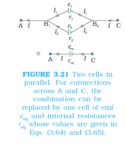
`color{blue} ✍️` Next, consider a parallel combination of the cells (Fig. 3.21). `I_1` and `I_2` are the currents leaving the positive electrodes of the cells. At the point `B_1, I_1 ` and `I_2` flow in whereas the current `I` flows out. Since as much charge flows in as out, we have
`color{purple}{I = I_1 + I_2}`
.............(3.67)
`color{blue} ✍️` Let `V (B_1)` and `V (B_2)` be the potentials at `B_1` and `B_2`, respectively.
`color{blue} ✍️` Then, considering the first cell, the potential difference across its terminals is `V (B_1) – V (B_2)`. Hence, from Eq. (3.5)
`color{purple}{V ≡V (B_1 ) – V (B_2 )=ε_1 - I_1 r_1}`
...............(3.68)
`color{blue} ✍️` Points `B_1` and `B_2` are connected exactly similarly to the second cell. Hence considering the second cell, we also have
`color{purple}{V ≡V B –V B_2 =ε_2 – I_2 r_2}`
............(3.69)
`color {blue}{➢➢}`Combining the last three equations
`I = I_1 + I_2`
`color{blue}{= (ε_1-V)/(r_1) + (ε_2-V)/(r_2) = ((ε_1)/r_1) + (ε_2)/(r_2) - V (1/(r_2) + 1/(r_2))}`
..............(3.70)
`color {blue}{➢➢}` Hence, `V` is given by,
`color{purple}{V = (ε_1r_2+ε_2r_1)/(r_1+r_2) - I(r_1r_2)/(r_1+r_2)}`
............(3.71)
`color{blue} ✍️` If we want to replace the combination by a single cell, between `B_1` and `B_2,` of emf `ε_eq` and internal resistance `r_eq`, we would have
`color{purple}{V = ε_(eq) - I r_(eq)}`
...........(3.72)
`color{blue} ✍️` The last two equations should be the same and hence
`color{purple}{V = (ε_1r_2+ε_2r_1)/(r_1+r_2)}`
............(3.73)
`color{purple}{r_(eq)= (r_1r_2)/(r_1+r_2)}`
.............(3.74)
`color{blue} ✍️` We can put these equations in a simpler way,
`color{purple}{1/(r_(eq)) = 1/(r_1+1/(r_2)}`
.............(3.75)
`color{purple}{ε_(eq)/(r_(eq)) = (ε_1)/(r_1) + (ε_2)/(r_2)}`
............(3.76)
`color{blue} ✍️` In Fig. (3.21), we had joined the positive terminals together and similarly the two negative ones, so that the currents `I_1, I_2` flow out of positive terminals.
`color{blue} ✍️` If the negative terminal of the second is connected to positive terminal of the first, Eqs. (3.75) and (3.76) would still be valid with `ε_2 → –ε_2` Equations (3.75) and (3.76) can be extended easily. If there an n cells of emf `ε_1, . . . ε_n` and of internal resistances `r_1, . . . r_n` respectively, connected in parallel, the combination is equivalent to a single cell of emf `ε_(eq)` and internal resistance `r_(eq)`, such that
`color{purple}{1/(r_(eq)) = 1/(r_1) + ....... + 1/(r_n)}`
............(3.77)
`color{purple}{(ε_(eq))/(r_(eq)) = (ε_1)/(r_1) + ...+ (ε_n)/(r_n)}`
...........(3.78)
`color{blue} ✍️` Like resistors, cells can be combined together in an electric circuit. And like resistors, one can, for calculating currents and voltages in a circuit, replace a combination of cells by an equivalent cell.
`color{blue} ✍️` Consider first two cells in series (Fig. 3.20), where one terminal of the two cells is joined together leaving the other terminal in either cell free. `ε_1, ε_2` are the emf’s of the two cells and `r_1, r_2` their internal resistances, respectively. Let `V (A), V (B), V (C)` be the potentials at points `A, B` and `C` shown in Fig. 3.20.
`color{blue} ✍️` Then `V (A) – V` (B) is the potential difference between the positive and negative terminals of the first cell. We have already calculated it in Eq. (3.57) and hence,
`color{purple}{V_(AB) ≡V(A) –V(B) =ε_1 – I r_1}`
.........(3.60)
Similarly,
`color{purple}{V_(BC) ≡V (B) – V (C)=ε_2 – I r_2}`
..........(3.61)
`color{blue} ✍️` Hence, the potential difference between the terminals A and C of the combination
`V ≡ V(A) – V(C)= [V(A) - V(B) ] + [V (B) - V(C)]`
`color{purple}{= (ε_1+ε_2)-I (r_1+r_2)}`
.........(3.62)
`color{blue} ✍️` If we wish to replace the combination by a single cell between A and C of emf `ε_(eq)` and internal resistance `r_(eq)`, we would have
`color{purple}{V_(AC) = ε_(eq)– I r_(eq)}`
.............(3.63)
`color {blue}{➢➢}`Comparing the last two equations, we get
`color{purple}{ε_(eq) = ε_1 + ε_2}`
.............(3.64)
and
`color{purple}{r_(eq) = r_1 + r_2}`
..............(3.65)
`color{blue} ✍️` In Fig.3.20, we had connected the negative electrode of the first to the positive electrode of the second. If instead we connect the two negatives, Eq. (3.61) would change to `V_(BC) = –ε_2–Ir_2` and we will get
`color{purple}{ε_(eq) = ε_1 – ε_2 (ε_1 > ε_2)}`
...........(3.66)
`color{blue} ✍️` The rule for series combination clearly can be extended to any number of cells:
`color{blue} {(i) }`The equivalent emf of a series combination of n cells is just the sum of their individual emf’s, and
`color{blue} { (ii)}` The equivalent internal resistance of a series combination of n cells is just the sum of their internal resistances.
`color{blue} ✍️` This is so, when the current leaves each cell from the positive electrode. If in the combination, the current leaves any cell from the negative electrode, the emf of the cell enters the expression for `ε_eq` with a negative sign, as in Eq. (3.66).
`color{blue} ✍️` Next, consider a parallel combination of the cells (Fig. 3.21). `I_1` and `I_2` are the currents leaving the positive electrodes of the cells. At the point `B_1, I_1 ` and `I_2` flow in whereas the current `I` flows out. Since as much charge flows in as out, we have
`color{purple}{I = I_1 + I_2}`
.............(3.67)
`color{blue} ✍️` Let `V (B_1)` and `V (B_2)` be the potentials at `B_1` and `B_2`, respectively.
`color{blue} ✍️` Then, considering the first cell, the potential difference across its terminals is `V (B_1) – V (B_2)`. Hence, from Eq. (3.5)
`color{purple}{V ≡V (B_1 ) – V (B_2 )=ε_1 - I_1 r_1}`
...............(3.68)
`color{blue} ✍️` Points `B_1` and `B_2` are connected exactly similarly to the second cell. Hence considering the second cell, we also have
`color{purple}{V ≡V B –V B_2 =ε_2 – I_2 r_2}`
............(3.69)
`color {blue}{➢➢}`Combining the last three equations
`I = I_1 + I_2`
`color{blue}{= (ε_1-V)/(r_1) + (ε_2-V)/(r_2) = ((ε_1)/r_1) + (ε_2)/(r_2) - V (1/(r_2) + 1/(r_2))}`
..............(3.70)
`color {blue}{➢➢}` Hence, `V` is given by,
`color{purple}{V = (ε_1r_2+ε_2r_1)/(r_1+r_2) - I(r_1r_2)/(r_1+r_2)}`
............(3.71)
`color{blue} ✍️` If we want to replace the combination by a single cell, between `B_1` and `B_2,` of emf `ε_eq` and internal resistance `r_eq`, we would have
`color{purple}{V = ε_(eq) - I r_(eq)}`
...........(3.72)
`color{blue} ✍️` The last two equations should be the same and hence
`color{purple}{V = (ε_1r_2+ε_2r_1)/(r_1+r_2)}`
............(3.73)
`color{purple}{r_(eq)= (r_1r_2)/(r_1+r_2)}`
.............(3.74)
`color{blue} ✍️` We can put these equations in a simpler way,
`color{purple}{1/(r_(eq)) = 1/(r_1+1/(r_2)}`
.............(3.75)
`color{purple}{ε_(eq)/(r_(eq)) = (ε_1)/(r_1) + (ε_2)/(r_2)}`
............(3.76)
`color{blue} ✍️` In Fig. (3.21), we had joined the positive terminals together and similarly the two negative ones, so that the currents `I_1, I_2` flow out of positive terminals.
`color{blue} ✍️` If the negative terminal of the second is connected to positive terminal of the first, Eqs. (3.75) and (3.76) would still be valid with `ε_2 → –ε_2` Equations (3.75) and (3.76) can be extended easily. If there an n cells of emf `ε_1, . . . ε_n` and of internal resistances `r_1, . . . r_n` respectively, connected in parallel, the combination is equivalent to a single cell of emf `ε_(eq)` and internal resistance `r_(eq)`, such that
`color{purple}{1/(r_(eq)) = 1/(r_1) + ....... + 1/(r_n)}`
............(3.77)
`color{purple}{(ε_(eq))/(r_(eq)) = (ε_1)/(r_1) + ...+ (ε_n)/(r_n)}`
...........(3.78)